Epidemic curves – Outbreak Toolkit

Overview

An epidemic curve (or epi curve) is a histogram (bar chart) that shows the distribution of cases over time. The time intervals are displayed on the x axis (the horizontal axis), and case counts are displayed on the y axis (the vertical axis). The result is a visual representation of illness onset in cases associated with an outbreak. The epi curve is an essential tool in an outbreak investigation and a key feature of descriptive epidemiology. It can provide useful information on the size, pattern of spread, time trend, and exposure period of the outbreak, and is often included in the epidemiological (epi) summary. The epi curve should be continuously updated as the outbreak progresses.

Basic epi curves

Whether creating an epidemic curve on paper or in a software program, these are important things to consider:

Plot the number of cases for each date/time on the graph. Include pre-outbreak time to show visually when the outbreak began. Since the epi curve is depicting a continuous variable, the bars should touch each other (unless there are periods of time with no cases).
Clearly label the x-axis (date/time of illness onset) and the y-axis (number of cases).
Give the epi curve a title that provides enough detail so that the figure can stand alone.
If depicting any cases other than confirmed cases (e.g., probable, suspect cases), these should be differentiated on the epi curve.

Advanced epi curves

Epi curves can be a powerful way to tell a meaningful story about the outbreak, even without lengthy text to explain the figure. While the general structure of epi curves are similar, there are ways to use the outbreak data to enhance the message.

Using different scales for the x-axis

The unit of time on the x-axis is usually based on the incubation period of the disease and the length of time over which cases are distributed. For example, for a disease with a short incubation period (e.g., Bacilius cereus) and cases distributed over a short period of time (hours), the scale for the x-axis may be more meaningful by hour rather than by day. Several epi curves with different units on the x-axis can be drawn to determine which portrays the data best. This is particularly useful when the disease and/or incubation is unknown.

Dealing with missing onset dates

A case may have many dates associated with their illness: illness onset date, report date, hospital admission date, specimen collection date, laboratory testing date, etc. While the general practice is to use illness onset date for all cases, these may not be readily available – for example, when a case could not be reached for an interview. To address this issue, the earliest available date for the case should be used to approximate the case’s illness onset.

The epi curve should clearly indicate in the footnotes that a set of criteria to establish an estimate has been used. As new information becomes available (e.g., updated dates), the epi curve should be updated with the earliest dates available (illness onset date, specimen collection date, received date, isolation date, report date).

Stratification – separating cases into categories

For some outbreaks, cases can be stratified (or separated) in the epi curve to help the reader understand the outbreak, particularly when there may be an interesting difference between the groups. There are often many ways to organize or separate outbreak cases into categories, such as:

Exposures (e.g., those who attended an event versus those that did not)
Geography (e.g., place of residence, patient location on hospital ward)
Personal characteristics (e.g., occupation – health care staff versus non-health care staff)

For example, the first epi curve includes all cases in one group by illness onset. The second epi curve stratifies cases by patient location on the hospital ward.

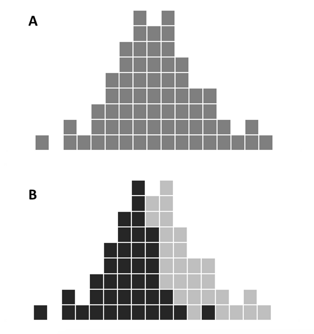
In this case, the stratification shows that the outbreak began on hospital ward A first (illness onset of patients on ward A were earlier than ward B). Being able to visualize the data in this way can help you hypothesize or understand key questions about the outbreak, such as how the pathogen is being transmitted from one ward to another.

Events of significance to the outbreak

Key events that occur during an outbreak can be added to the epi curve as a way to tell a more comprehensive story about why cases are distributed in a particular way. The timing of these events may help describe visible changes on the epidemic curve. Some examples include:

Exposures (e.g., mass gathering event, implicated dinner)
Public health measures (e.g., restaurant closure, product recall)
Communications (e.g., media release warning public not to consume implicated food)

These events can be incorporated onto the epi curve using text boxes and arrows. However, it is important to keep in mind that the overall epi curve should still remain simple and easy to understand.

Analysing an epi curve

As well as visually depicting distribution of cases over time, the epi curve can tell investigators a number of other things about the outbreak. These include: size, time trend, outliers, and pattern of spread.

Size

The size of your epidemic curve can help validate whether you are in an outbreak by showing an increased number of cases over the baseline visually. Knowing the number of cases affected may also help you generate and refine your hypothesis.

Time trend

The epi curve can provide information on the progression of the outbreak (e.g., if the outbreak is ongoing, increasing in size, stabilizing, decreasing, over, etc.). The epi curve will also depict the rate of increase or decrease of cases over time. When you are at a point where you would like to declare the outbreak over, it is important to ensure that the decline in cases is a true decrease and not due to a reporting delay. As there are inherent delays between when a case becomes ill and the date that public health is aware of the case, this means that the full picture of the outbreak will not be available, particularly for the most recent time period (e.g., days).

Outliers

The outbreak curve can also identify outliers – cases that stand apart from the overall pattern such as the first, or index case thereby providing important clues about the source of the outbreak. Outliers can also result from secondary transmission.

Pattern of spread

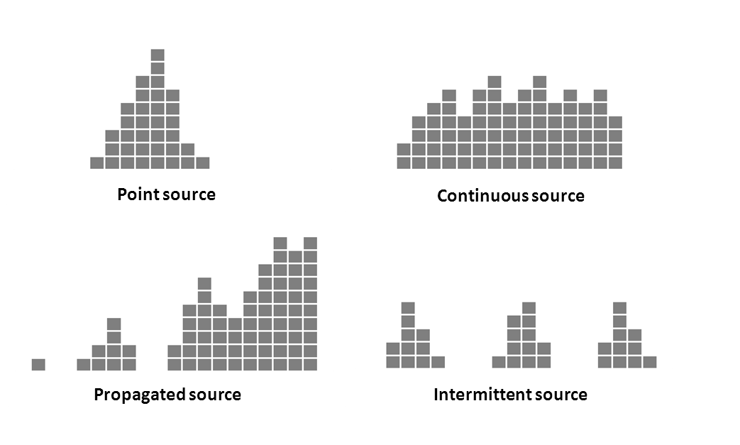
The overall shape of the epi curve may help identify the mode of transmission of the outbreak. There are several well-described types of epi curves: point source, continuous common source, propagated source, and intermittent source.

Point source – Persons are exposed to the same common source over a brief period of time, such as through a single meal or event attended by all cases; number of cases rise rapidly to a peak and falls off gradually; majority of cases occur within one incubation period.
Continuous source – Exposure is not confined to one point in time (prolonged over a period of days, weeks or longer); as such, cases are spread over a greater period of time depending on how long the exposure persists; lasts more than one incubation period
Propagated source – does not have a common source but instead caused by spread of pathogen from one susceptible person to another; transmission may occur directly (person-to-person) or via an intermediate host; tends to have a series of irregular peaks reflecting the number of generations of infection; multiple peaks separated by approx. one incubation period; e.g., person-to-person spread of shigellosis
Intermittent source – similar to continuous but exposure is intermittent; multiple peaks – length: no relation to the incubation period (reflects intermittent times of exposure) e.g., contaminated food product sold over period of time

The shape of an epidemic curve will rarely fit any of these descriptions exactly, but can still provide a general sense of the pattern of spread. In some cases for example, the outbreak type is a mixed outbreak pattern, which can involve both a common source outbreak and secondary propagated spread to others (usually household members). Many foodborne pathogens (such as Norovirus, hepatitis A, Shigella and E. coli) commonly exhibit this mode of spread.

Further reading: Association of Faculties of Medicine of Canada. AFMC Primer on Population Health, Patterns of disease development in a population: the epidemic curve.

Examples

Tools

Toolkit epi curve exercise

This exercise shows how to make an epidemic curve in Microsoft Excel, where each case is represented by a single box using this data set.

Toolkit pivot tables exercise

This exercise uses an outbreak line list to create PivotTables in Microsoft Excel and use them to extract information for descriptive epidemiological summaries and create epidemic curves.

Toolkit line list and data dictionary

This Microsoft Excel-based tool is designed to be used as a template for foodborne outbreak investigation line lists. Once data has been entered, common descriptive statistics are automatically calculated. A data dictionary describing each data field in the line list is available in the final tab.

On this page